You were looking for what? (Or, search term questions.) October 26, 2017
Posted by tomflesher in Macro, Teaching.Tags: CPI, Reader questions
1 comment so far
Occasionally I mine the search terms for interesting questions. Here are three from the past month:
- What is an increase in CPI?
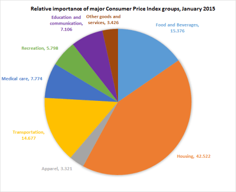 When a country’s CPI increases, that means that, on average, the cost of living in the country has increased. The Consumer Price Index measures the price of a fixed basket of goods. For example, in the United States, CPI consists largely of housing costs, food and beverages, and transportation. When the price of any good in the basket goes up, it increases total basket expenditure, but the effects of (for example) increasing food costs would be greater than the effects of increasing costs of haircuts (included in the “Other” category). Although the BLS is careful to point out that the CPI is not a cost-of-living index, it functions a lot like one. (The chart was retrieved from the US Department of Labor website.)
The percentage change in CPI, otherwise called the CPI growth rate, is the most common measure of inflation.
- if the cpi went up why not all the goods prices goes up? [sic]
This question gets the causation backwards. The CPI measures how much prices are changing; you can use the percentage change in CPI to measure how much, on average, prices have gone up, but that says very little about individual goods. For example, the Transportation category includes the price of gasoline. If cell phone bills decreased, but gasoline prices increased, the fact that we (on average) spend more money per year on gasoline than on phone bills (as reflected by the different weights, above) means that the gas price increase will have a greater effect on our overall spending.
CPI reflects those changes. It’s possible for the total cost of the basket of goods used to measure CPI to increase even if some of those goods had steady or even decreasing prices.
- mastovesion is good or bad
You do you, gentle reader.
Faculty Freebies and Price Discrimination April 3, 2017
Posted by tomflesher in Examples, Micro, Teaching.Tags: Introduction to Microeconomics, Price discrimination, Principles of Microeconomics
add a comment
Despite its nasty-sounding name, price discrimination is interesting and beneficial to some consumers. (Of course, when we move away from equilibrium to make someone better off , we usually make some other consumers worse off.)
Textbook publishers face a classic case where price discrimination would be useful: they want to charge students high prices for their textbooks, but because professors have the power to require a textbook of their students, they want to get professors on board as easily as possible. That usually means lowering the price of the book for professors (to make it easy to get); I get tons of free books every semester.
Publishers don’t want those free books to get into students’ hands, though – that means either a student didn’t pay for a book because a virtuous professor gave a freebie away, or the student paid, but paid an unscrupulous professor for a book the professor got for free! If a student is going to pay for a book, the publisher would rather get a cut of it.
Goods that are difficult to resell are easiest to discriminate on. Publishers have, for a long time, printed “INSTRUCTOR’S REVIEW COPY – NOT FOR SALE” on books. That has some effect, but you still have the possibility of paying for a book on Amazon or AbeBooks. One way to keep students from buying these books is to sink money into online resources, which are tied to students’ identities. That way, even if the student buys a used copy of the physical text, they still have to pay for access to the online resources. Still, not every instructor uses those, so this isn’t foolproof.
One publisher, Cengage, has taken an additional step with Greg Mankiw’s principles book: not only does it say “Compliments of N. Gregory Mankiw” on the front, along with the usual “Instructor’s Edition” language, it has my name embossed on the cover. “Specifically prepared for” is printed, and “Thomas Flesher” is stamped into the front cover. (Of course, I prefer Tom, but you can’t be too picky with freebies.) This is a pretty clever means to keep me from reselling the book, at least unless I have a high name value. I can easily imagine a student wanting to purchase a book specifically prepared for Dean Karlan or Paul Krugman, for example, if either of them still teaches Principles using Greg’s book. (I doubt it, since each of them has his own.)
Either way, Cengage is trying to protect what’s likely its largest profit-producer by minimizing the number of free copies students can use.
How do producers charge different consumers different prices? September 29, 2015
Posted by tomflesher in Micro, Teaching.Tags: Introduction to Microeconomics, micro, Microeconomics, Price discrimination, Principles of Microeconomics
add a comment
Price discrimination is the act of charging different consumers different prices based on how much they’re willing to pay. There are a few different forms of price discrimination, and it can be achieved different ways depending on how much information a seller has.
Haggling, or negotiating to find an exact willingness to pay, is an effective form of price discrimination for large purchases. For example, a car salesman can often start with a high price, and when the customer refuses, he can incrementally lower the price (or otherwise adjust the offer) until he find a deal that the buyer is just barely willing to accept. This has one huge advantage – it gets the most that the customer is willing to give up (or, in other words, it extracts the customer’s maximum willingness to pay). It is, however, very costly for a salesman. Just imagine if the salesman were to spend a whole day negotiating only to realize the buyer wasn’t willing to pay enough to cover the cost of the car. Then, the salesman loses the chance to make a sale at all that day. Since it’s costly, this method is most useful for high-priced items like cars and houses.
If you ask a consumer what he’s willing to pay, he’ll lowball you; haggling helps force the price (and the profit) up.
Direct segmentation allows a market to be broken up based on some visible characteristic. In the previous post, I discussed my father-in-law’s senior citizen discount on haircuts and how he pays less than I do for the same cut. He does this by asking for a senior citizen discount, which I’m not eligible for.
Direct segmentation involves breaking the market up into different groups and intentionally charging different prices to those different kinds of people. It works best when one group has a higher willingness to pay – so, since I’m not a college student, and not a senior citizen, my (relatively) high income means I don’t ask for a discount. Similarly, I pay a lower price to have my blazers dry-cleaned than my department chair does, even though her blazers are made up of a smaller amount of fabric. Dry-cleaners just automatically charge a higher price for a woman’s garment than a man’s, even if the garment is similar.
This sometimes leads to unpleasant outcomes. NPR did a story on a 12-year-old girl who had to pay a premium to play Temple Run as a female character; non-white-male characters were all in-app purchases that cost money.
Indirect segmentation is like direct segmentation, but requires the consumer to do some work to get the lower price. A good example of this would be a volume discount. I have a strong preference for Crayola An Du Septic dustless chalk. (I like its weight and erasability.) When I purchase chalk to use in the classroom, my buying options include paying about $3.50 for a single box or about $12 for a 12-box package. No sane person who isn’t a teacher has any use for 12 boxes of blackboard chalk, so I signal my price sensitivity by buying a larger amount at once.
Another way people reveal their types is by clipping coupons. A coupon is like a little badge that says “I’m cheap! Give me a lower price!” By doing a bit of extra work to signal my cheapness, I qualify myself for a lower price just as much as if I’d haggled with the guy behind the counter.
Price Discrimination September 28, 2015
Posted by tomflesher in Micro, Teaching.Tags: industrial organization, micro, Microeconomics, Price discrimination, Principles of Microeconomics
2 comments
I wear my hair short. Like, really short – it’s buzzed on the sides and scissor-cut on top, so that it’s low-maintenance, and I trim my own beard using a storebought clipper. My father-in-law does the same thing – except he pays a little bit less than I do, because he tells the barber he’s old and cheap. Why does that work?
A business, we assume, wants to make money. As such, it wants to sell its good at the highest price possible to each consumer. Consumers, though, want to spend as little as possible, to maximize the difference between their willingness to pay and the actual price they pay. (Economists call that difference consumer surplus.) Most of the time, it’s difficult to charge people different prices based on their willingness to pay. To do so requires three big elements.
First, the market has to be segmented. This means that consumers have to have different willingnesses to pay. Think about a price-sensitive consumer like my father-in-law – he’s getting ready to retire. His wife is already retired. He needs to adjust to spending less money than he’s used to. A lot of his fellow senior citizens feel his pain. Meanwhile, I’m a young(ish) guy. I teach at a community college, I have no kids, and I have a long time before I retire (so my money has a lot of time to grow). I’m willing to pay a little bit more for a haircut than he is. In addition to senior citizens, college students are often given discounts just for being students.
Second, there needs to be some element of monopoly power. My barber isn’t a monopolist, because pure monopoly is rare, but I do go out of my way to go to a place where I have a good rapport with the barber. I have a guy who cuts my hair the way I like it, and I like the atmosphere at his shop. Plus, even though I could probably shop around to find a cheaper price if I went somewhere else, I couldn’t find a price that much cheaper. Haircuts have pretty standard prices around here. That’s what the monopoly power condition is intended to enforce – if I get angsty about not getting a cheap haircut, I don’t really have other options.
Finally, the good needs to be difficult to resell. If we were talking about an oil change on my car, I might send my father-in-law into the mechanic’s shop with my car to get the senior citizen discount on an oil change. When we have a family event planned, he buys the bagels because the local place gives him a deal just for being older. Or if my mother is looking to redo the bathroom, or kitchen – my father has friends at http://www.restorationusa.com/west-palm-beach/ who’ll give them a great discount on that as well. It’s impossible, though, to resell a haircut, so I can’t use his senior citizen discount to my advantage here. Baseball and hockey tickets often offer student rush specials where you have to (theoretically) show a student ID to get the discount. Enforcing that would ensure that people with high willingness to pay didn’t buy the cheap tickets in the nosebleed section, but the open secret is that the Mets don’t really care if you buy cheap tickets, as long as you buy tickets.
If those three conditions exist, then it’s possible for a seller to charge different people different prices. Economists call that price discrimination. It’s not necessarily a bad thing, though – it means if you’re cheap, you can get a pretty good deal on some goods.
Diminishing Marginal Returns September 9, 2015
Posted by tomflesher in Micro, Models, Teaching.Tags: diminishing marginal returns, graphs, Sriracha
add a comment
Close your eyes.
Well, finish reading the next paragraph first, and then close your eyes.
I am going to offer you unlimited access to something good, something useful, something tasty. That’s right – I’m going to let you have as big a bottle as you’d like of Sriracha. As long as you can carry it away, you can put as much Sriracha as you’d like on your plate of pad thai and I won’t look askance at you. No, I might even respect you. How much are you going to take?
Open your eyes.
The funny thing about that thought experiment is that everyone can picture how much they’d put on a plate of noodles. Some people might put none at all;1 others might put a little dab on the side, while still others, possibly economics professors who operate multiple blogs with self-deprecating titles, might put a truly ridiculous amount and allow the streets to run red with the blood of the non-rooster-sauces. Almost no one would ever take an unlimited amount of sauce.
That’s because, like most goods, Sriracha demonstrates diminishing marginal returns. That means that if Sriracha is meant to create tastiness, then for every extra drop of Sriracha, the tastiness increases, but the increase gets smaller. Mathematically, that means the slope is positive, but decreasing; that’s the same as saying the function has a positive first derivative and a negative second derivative. One common function used to model diminishing marginal returns is the natural log function, y = ln(x). If we assume that tastiness is logarithmic in grams of Sriracha, the graph might look like this:
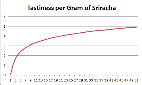 Just about any good demonstrates diminishing marginal returns, and at some point you’ll have enough of a good that its marginal benefit no longer exceeds its marginal cost.
—–
1 Those people are called wimps.
Elasticity and Demand March 18, 2015
Posted by tomflesher in Micro, Teaching.Tags: demand, elasticity, intermediate microeconomics, Introduction to Microeconomics, micro, Microeconomics, Principles of Microeconomics
add a comment
The price-elasticity of demand measures how sensitive consumers are to changes in price. There are two primary formulas for that. Most commonly, introductory courses will use 


A graph of demand and price-elasticity of demand
Take note of the shape of that formula, and keep in mind the Law of Demand, which states that as price increases, quantity demanded decreases. At high prices, quantities are relatively low, meaning that a small change in price yields a relatively big change in quantity demanded. If the percentage change in quantity demanded is bigger than the percentage change in price, then demand is elastic and consumers are price-sensitive. On the other hand, at low prices, quantities are relatively high, meaning that a small change in price yields an even smaller change in quantity demanded. That means demand is inelastic.
This pattern of high prices corresponding to elastic demand and low prices corresponding to inelastic demand holds for most goods. At a very high price, firms can make a small change in price to try to encourage new buyers to buy their product, whereas at a very low price, firms can jiggle the price up a little bit to try to snap up some extra revenue without dissuading most of their buyers from purchasing the product.
A slightly more accurate formula for price-elasticity of demand is 
The graph in this post shows market demand 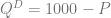
The Do-Nothing Alternative March 16, 2015
Posted by tomflesher in Examples, Micro, Teaching.Tags: Do-Nothing Alternative, hidden choices, opportunity cost
add a comment
Consider the following situation: You are at a casino. You have a crisp new $100 bill in your pocket and an hour before your friend arrives. There are several options available: blackjack, poker, and slot machines. Each has its advantages and disadvantages. Blackjack offers a 45% probability that you will double your money over the next hour, but a 55% probability you will lose it all. Based on your understanding of statistics, you know this means you should expect to have about $90 at the end of the hour. Poker is a better proposition – since it is a game of skill, you have a 60% chance of earning an extra $50 (for a total of $150), but a 40% chance of losing all of your money. That means you can expect to have about $90 in your pocket at the end of the hour. Slot machines, to go to the other extreme, are a highly negative expected-value proposition. You stand a 1% chance of winning $1000, but a 99% chance of losing all of your money. As a result, you could expect to have about $1 in your pocket at the end of the hour.
Thinking like an economist, you quickly winnow your options down to blackjack or poker, since you cannot abide such a risky proposition. Then, however, you’re stuck – the expected values are the same. Which game is it rational to play?
Similarly, consider this problem raised in a freshman course on ethics: You are on your way out of a coffee shop carrying a double shot of espresso and a $1 bill you received as change. Two homeless people, one man and one woman, each step toward you and simultaneously ask you for the dollar. Since you don’t have any coins, you cannot split the value between the two people. Who should you give your dollar to?1
What do these two situations have in common? In each of them, you are attempting to choose between two options that result in negative consequences for you. In the gambling scenario, you have two options, each with the expectation of losing $10. In the coffee shop scenario, you have two people each asking for $1. In neither case is there a compelling reason to choose one option over the other. The underlying assumption, though, is that we must choose an option at all.
The do-nothing alternative is often (but not always) a hidden option when making choices. For example, in the gambling scenario, you have the option to literally do nothing for an hour until your friend arrives. This leaves you $100 with certainty. In the coffee shop scenario, you have the option to politely refuse each person’s request, leaving you free to keep your dollar. Not every situation allows a do-nothing option; for example, a baseball manager faced with the option of starting his worst starting pitcher or a pitcher who is usually used only in long relief cannot opt to simply start no pitcher. However, a voter who is disgusted with all available candidates may bemoan his “forced” vote for the lesser of two evils without acknowledging that he has the option simply not to vote at all. The do-nothing option is often low-cost but has low returns as well, making it a great way to avoid choosing the best of a bad lot, but a lousy choice for a firm seeking growth.
—–
1 This was met with considerable debate about the probability that the homeless woman had children.
The Good and Bad of Goods and Bads January 25, 2015
Posted by tomflesher in Micro, Teaching, Uncategorized.Tags: economics, intermediate microeconomics, Introduction to Microeconomics, Microeconomics, preferences, Principles of Microeconomics
add a comment
When students first hear the word “goods” pertaining to economic goods, they sometimes find it a little funny. When they hear some sorts of goods called “bads,” they usually find it ridiculous. Let’s talk a little about what those words mean and how they pertain to preferences.
Goods are called that because, well, they’re good. Typically, a person who doesn’t have a good would, if given the choice, want it. Examples of goods might be cars, TVs, iPads, or colored chalk. Since people want this good if they don’t have it, they’d be willing to pay for it. Consequently, goods have positive prices.
That doesn’t mean that everyone wants as much of any good as they could possibly have. When purchasing, people consider the price of a good – that is, how much money they would have to spend to obtain that good. However, that’s not because money has any particular value. It’s because money can be exchanged for goods and services, but you can only spend money once, meaning that buying one good means giving up the chance to buy a different one.
Bads are called that because they’re not good. A bad is something you might be willing to pay someone to get rid of for you, like a ton of pollution, a load of trash, a punch in the face, or Taylor Swift. Because you would pay not to have the bad, bads can be modeled as goods with negative prices.
Typically, a demand curve slopes downward because of the negative relationship between price and quantity. This is true for goods – as price increases, people face an increasing opportunity cost to consume one more of a good. If goods are being given away for free, people will consume a lot of them, but as the price rises the tradeoff increases as well. Bads, on the other hand, act a bit different. If free disposal of trash is an option, most people will not keep much trash at all in their apartments. However, as the cost of trash disposal (the “negative price”) rises, people will hold on to trash longer and longer to avoid paying the cost. Consider how often you’d take your trash to the curb if you had to pay $50 for every trip! You might also look to substitutes for disposal, like reusing glass bottles or newspaper in different ways, to lower the overall amount of trash you had to pay to dispose of.
As the cost to eliminate bads increases, people will suffer through a higher quantity, so as the price of disposal increases, the quantity accepted will also increase.
Don’t Discount the Importance of Patience April 9, 2013
Posted by tomflesher in Micro, Teaching.Tags: discount rates, interest, interest rates
1 comment so far
Uncertainty is one explanation for why interest rates vary. Tolerance for uncertainty is called risk aversion, and it can be pretty complicated. (We’ll talk about it a little bit later on.) Another big concept is patience. Willingness to wait is also pretty complicated, but that’s our topic for today.
It’s easy to imagine some reasons that people would have different levels of patience. For one, you’d expect a healthy thirty-year-old (named Jim) to be more patient than a ninety-year-old (named Methuselah). What if someone (named Peter) offered us a choice between $100 today or a larger amount of money a year from now? How much would it take for Jim and Methuselah to take the delayed payoff? Would they take $100 a year from now? A lot can change in a year:
- There could be a whole bunch of inflation, and the $100 will be worth less next year than it is now. Boom, we’ve lost.
- We could put the money in the bank and earn a few basis points of interest. Boom, we’ve lost.
- We could die and not be able to pick up the money. Boom, we’ve lost.
- Peter could die and we wouldn’t be able to collect. Boom, we’ve lost.
Based on these, we’ll want a little bit more money next year than this year in order to be willing to take the money later instead of the money now. Statistically, though, Jim is more likely than Methuselah to be there to pick up the money.
Neither would take any less than $100 next year, but that’s just a lower limit. According to Bankrate.com, Discover Bank is paying 0.8% APY, which means that the $100 would be worth .8% more next year – just by putting the money in the bank, we can trade the risk that the bank goes bust (really unlikely) for the risk of Peter dying. That’s an improvement in risk and an improvement in payoff, so there’s no reason to take any less than $100.80. Again, though, this is a lower bound. Peter still has to pay for making them wait. That’s where the third point comes into play.
Methuselah is probably not going to live another year. It’s much more likely that he’ll get to spend the $100 than whatever he gets in a year; in order to make it worth the wait, the payoff would have to be huge. Methuselah views money later as worth a lot less than money today. He might need $200 to make it worth the wait. Jim, on the other hand, might only need $125. He has more time, so he’s much more patient.
This level of patience is called a discount rate and is usually called β. You can do this sort of experiment to figure out someone’s patience level. You’d then be able to set up an equation like this, where the benefit is the $100 and the cost is what you give up later:

Methuselah, then, would have

so β = 1/2.
Jim would have the following equation:

so β = 4/5.
Based on this, we can say that Methuselah values money one year from now at 50% of its current value, but Jim values money one year from now at 80% of its current value. Everyone’s discount rate is going to be a little bit different, and different discount rates can lead people to make different choices. If Peter offers $100 today or $150 tomorrow, Jim will wait patiently for $150. Methuselah will jump at the $100 today. Both of them are rational even though their choices are different.
Evaluating Different Market Structures December 13, 2012
Posted by tomflesher in Micro, Teaching.Tags: consumer surplus, Cournot, equilibrium, intermediate microeconomics, Introduction to Microeconomics, market week, monopoly, perfect competition, perfectly competitive markets, profit, welfare
add a comment
Market structures, like perfect competition, monopoly, and Cournot competition have different implications for the consumer and the firm. Measuring the differences can be very informative, but first we have to understand how to do it.
Measuring the firm’s welfare is fairly simple. Most of the time we’re thinking about firms, what we’re thinking about will be their profit. A business’s profit function is always of the form
Profit = Total Revenue – Total Costs
Total revenue is the total money a firm takes in. In a simple one-good market, this is just the number of goods sold (the quantity) times the amount charged for each good (the price). Marginal revenue represents how much extra money will be taken in for producing another unit. Total costs need to take into account two pieces: the fixed cost, which represents things the firm cannot avoid paying in the short term (like rent and bills that are already due) and the variable cost, which is the cost of producing each unit. If a firm has a constant variable cost then the cost of producing the third item is the same as the cost of producing the 1000th; in other words, constant variable costs imply a constant marginal cost as well. If marginal cost is falling, then there’s efficiency in producing more goods; if it’s rising, then each unit is more expensive than the last. The marginal cost is the derivative of the variable cost, but it can also be figured out by looking at the change in cost from one unit to the next.
Measuring the consumer’s welfare is a bit more difficult. We need to take all of the goods sold and meausre how much more people were willing to pay than they actually did. To do that we’ll need a consumer demand function, which represents the marginal buyer’s willingness to pay (that is, what the price would have to be to get one more person to buy the good). Let’s say the market demand is governed by the function
QD = 250 – 2P
That is, at a price of $0, 250 people will line up to buy the good. At a price of $125, no one wants the good (QD = 0). In between, quantity demanded is positive. We’ll also need to know what price is actually charged. Let’s try it with a few different prices, but we’ll always use the following format1:
Consumer Surplus = (1/2)*(pmax – pactual)*QD
where pmax is the price where 0 units would be sold and QD is the quantity demanded at the actual price. In our example, that’s 125.
Let’s say that we set a price of $125. Then, no goods are demanded, and anything times 0 is 0.
What about $120? At that price, the quantity demanded is (250 – 240) or 10; the price difference is (125 – 120) or 5; half of 5*10 is 25, so that’s the consumer surplus. That means that the people who bought those 10 units were willing to pay $25 more, in total, than they actually had to pay.2
Finally, at a price of $50, 100 units are demanded; the total consumer surplus is (1/2)(75)(100) or 1875.
Whenever the number of firms goes up, the price decreases, and quantity increases. When quantity increases or when price decreases, all else equal, consumer surplus will go up; consequently, more firms in competition are better for the consumer.
Note:
1 Does this remind you of the formula for the area of a triangle? Yes. Yes it does.
2 If you add up each person’s willingness to pay and subtract 120 from each, you’ll underestimate this slightly. That’s because it ignores the slope between points, meaning that there’s a bit of in-between willingness to pay necessary to make the curve a bit smoother. Breaking this up into 100 buyers instead of 10 would lead to a closer approximation, and 1000 instead of 100 even closer. This is known mathematically as taking limits.
