Money Neutrality (or, the Quantity Equation) March 4, 2011
Posted by tomflesher in Macro, Teaching.Tags: economics, Introduction to Macroeconomics, macro, macroeconomics, Money neutrality, mv = py, Principles of Macroeconomics, quantity equation
2 comments
The Macro class I’m TAing has just gotten to money growth and inflation, chapter 12 in Mankiw’s Brief Principles of Macroeconomics. As usual, the quantity equation, MxV = PxY, confuses some of the students a little bit, so I thought I’d see what I can do to clarify it a little.
First, let’s define some terms. M is the size of the (nominal) money supply. V is the velocity of money, or the number of times a given dollar is spent in a year. (It represents how fast people spend money, so that if the money supply is only $100 but GDP, the total of expenditures on all final goods and services in the US in a year, is $500, the velocity of money is 5/year.) P is the nominal price level – that is, just the average price of stuff in the economy. Y is real GDP, so it represents the production level or the amount of stuff produced in the economy.
For reasons of a mathematical nature1 explained at the end of the page, you can think of PxY as all of the expenditures in the economy, and because of that, you can think of it as the product of the average price and the quantity produced. So, the right-hand side of the quantity equation is nominal GDP.
V is determined by many different things. For example, when people feel less confident about the economy, V might drop because people would spend less money. When people feel more confident, they spend more easily, and so V might rise. A lot of things that affect V are difficult to talk about if we only have Principles-level tools, though, so the conventional wisdom is to leave V constant for now.
Then, we basically have the equation:

What this means is that a change in the money supply has to be matched by the change in price level and the change in production.2 If all we know is that the money supply changed, then it could be due to a change in the price level, a change in real production, or some combination of the two. If on the other hand the price level changes and production doesn’t, then it must be due to a change in the money supply (like if the government started printing too much money).
When there’s too much money in the economy, price levels rise; when businesses produce more, then the real GDP level (Y) will increase, so if the money supply doesn’t increase then price levels would be expected to fall3; when price levels are changed for some outside reason, then either GDP has to change, the money supply has to change, or both.
Note:
1 Under the expenditure method, the Gross Domestic Product or GDP is the total market value of all final goods and services produced in the economy in a given period of time. For each good or service, it will either be recorded as a sale if someone buys it or as inventory by the business that produced it if it isn’t sold. So, for every good i in the economy with a given nominal price i, the contribution to GDP of that good is

So, in an economy with n goods, you can add up all of the expenditures on those goods and generate nominal GDP. Thus,

This is equivalent to multiplying the average price by the total number of goods in the economy.
2 This can be shown using the natural logarithm transformation. Since the interpretation of a change in the natural logarithm is the percentage change in the untransformed variable,


So, the percentage change in M can be decomposed into two pieces: the percentage change in P and the percentage change in Y.
3Thanks to Roman Hocke for catching an error in an earlier version of this post.
Beerflation February 26, 2011
Posted by tomflesher in Macro, Teaching.Tags: Big Mac Index, purchasing power, purchasing power parity, real prices
add a comment
One of the ways we measure well-being is through purchasing power. There are a lot of unusual measures of purchasing power; possibly the most famous is The Economist’s Big Mac Index, which measures the price of a Big Mac in different countries as a way of checking to see if reported exchange rates are correct.
This depends on idea of purchasing power parity. That is, if we’re going to compare prices in different currencies, the goods we’re comparing have to be precisely the same. The Big Mac is thus an ideal good to use for an exchange rate calculation since the point of branding McDonalds burgers is that they provide a consistent experience.
Another use of purchasing power is to estimate well-being across time periods. If your wage rose at a faster rate than the price level did, you’re better off than you used to be. James over at the Supine Bovine uses the rising price of beer relative to the minimum wage to illustrate that the average entry-level worker (personified as “twenty-somethings who are stuck living with mom and dad”) is worse off in the current economy than he used to be:
So I ask my dad what minimum wage was back in the day and what the price of beer (at a bar) was; he told me it was (about) $4/hour and $0.25, respectively. This means that on one hour of minimum wage work he could get shitfaced – 16 beers is no small amount. Anyway, today the minimum wage is $8/hour and a beer at a bar costs no less than $3.50 (but you’re looking at double that at most places). So my peers can purchase at most two beer per hour worked at minimum wage. So… beer costs about 8 – 16 times what it used to.
Now, I have a few quibbles with this (mainly to illustrate the problems with using a single good to compute inflation). For one, if That ’70s Show is any indication, bar beer hasn’t always been served in twelve-ounce containers. Adjusting down to an eight-ounce glass, that leaves us with approximately 12 beers. Second, are we discussing the same beer? Even moderate changes in alcohol content can adjust this calculation quite a bit. If, for example, James is using Labatt Blue at 5% alcohol by volume, then substituting the price of Sierra Nevada Pale Ale at 5.6% means that one Sierra Nevada is about 1.12 Blues. That kicks the old figure down to about 10.7 beers, or, equivalently, an old price of .09 hours worked for a beer. (Note that this doesn’t substantially change James’ point.) The current ratio, accepting James’ $3.50 figure as correct, is about .43 hours worked for a beer, meaning the real price of beer has risen approximately 386%. (When I say ‘real price,’ I am indicating that the price is expressed in terms of other goods, rather than in dollars.) It’s impossible to compute a rate of inflation because we don’t know what year James’ dad was talking about.
On the other hand, a lot of twenty-somethings these days have laptops. Just spitballin’.
A Worked Example on the Money Multiplier February 26, 2011
Posted by tomflesher in Macro, Teaching.Tags: fractional reserve banking, Money multiplier, t-account, worked examples
3 comments
In the previous post, I introduced the thinking underlying the Money Multiplier. It represents how money is created by the process of loaning money that’s held on deposit. A portion of the money on deposit must be held in reserve to make sure the bank can function. This is what’s called a fractional reserve banking system. This post will work with a standard problem setup that you might see on your Principles of Macroeconomics exam and show how to answer different questions that might be asked about it.
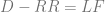
A bank’s balance sheet is usually expressed in the form of a T-account. On the left-hand side, assets are listed. On the right-hand side, liabilities are listed. Deposits are a liability because the bank must be prepared to pay them out at any time. I abbreviate Deposits as D. Similarly, because loans (abbreviated L) will be paid back (are receivable), they represent an asset. Any funds that the bank could lend are called loanable funds, abbreviated LF. Assets break down into two categories: loans and reserves.
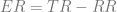
Reserves break down into two categories: required reserves and excess reserves. Required reserves are the fraction of deposits that banks are required by law to keep on hand; excess reserves are money on hand that are above the excess reserve amount. Using the convention that rr means reserve ratio, RR means required reserves, TR means total reserves, and ER means excess reserves, the following identities hold:


Take the following bank’s T-account:

The first thing that the exam might ask you is:
1. If the bank holds no excess reserves, what is the reserve ratio?
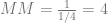
The question tells me that ER = 0, which means that RR = TR = $250. Since D*rr = RR, 1000 * rr = 250, dividing both sides by 1000 yields that rr = 250/1000. In lowest terms, this is 1/4, or .25 in decimal form.
2. If the reserve ratio is 1/10, what is the amount of excess reserves?
Begin with D = $1000. D*rr = RR, so $1000*1/10 = RR = $100. Then, since ER = TR – RR, ER = $250 – $100 = $150.
3. If the reserve ratio is 1/10, what is the largest new loan this bank could prudently make?
This is a tricky question because it’s simply a complicated way of asking how much the bank is holding in excess reserves. Why? Because a bank is allowed to loan out all but the required reserves. If a bank holds more than the required reserves, they have excess reserves (by definition) and they are allowed to loan out more money. Therefore, by the same method as question 2, the answer to this is $150.
4. Suppose the reserve ratio is 1/4. If the Fed lowers the reserve ratio to 1/5, what is the effect on the size of the money supply?
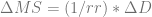
This requires two formulas from my previous entry, where I defined the Money Multiplier. Those formulas are


Here, the change in deposits 


Even if we don’t know the money supply, we know how much it will change from this bank.


So this small change in the required reserve ratio will lead to an increase in deposits of $200 from this bank.
Why is the Money Multiplier 1 over the Reserve Ratio? February 25, 2011
Posted by tomflesher in Macro, Teaching.Tags: Federal Reserve Bank, Introduction to Macroeconomics, macroeconomics, monetary policy, monetary theory, money creation, Money multiplier, Principles of Macroeconomics, reserve ratio
2 comments
Or, How does the banking system create money?
The Introduction to Macroeconomics class I’m TAing just got to the Monetary System. This was a difficult chapter for the students last semester, so I want to place a clear explanation online and give a mathematical proof for some of the more motivated students who look grumpy when I handwave away the explanation. For those who want to play with this themselves, I’ve created a spreadsheet that shows the process of money creation. You can choose an initial deposit and a reserve ratio (which I set at $1000 and 1/10), then trace out the changes as people borrow the money.
It boils down to what banks are for. The biggest mistake you, in your capacity as a consumer, can make is to think that the purpose of a bank is to give you a place to save money. Really, the purpose of a bank is to serve as a financial intermediary, which allows people who want to lend money (savers) to find people who want to borrow money (borrowers). When you put your money in a savings account, you’re putting money into the pool of loanable funds, and the bank will pay you a small amount of interest. Why don’t they let you do that yourself? Two reasons:
- They have more information about who wants to borrow money (specifically, businesses and consumers ask them for loan), and
- They offer a small return with certainty, whereas if you found a borrower yourself, you’d have to collect your return yourself.
In order to provide this certainty, the banks have to hold a certain amount of each deposit in reserve, in order to make sure that people who want to take their money out can do so. This is the reserve ratio, and it’s set by the Board of Governors of the Federal Reserve. Adjusting the reserve ratio upward means that a bank needs to hold a larger portion of each deposit, so they have less to lend out. That means that all things being equal, money will be harder to get than with a smaller reserve ratio, and so interest rates rise and less money is created. Conversely, lowering the reserve ratio means that banks have more money they can lend out and more money will be created.
When you deposit $1000 in the bank, if the reserve ratio is 1/10 or 10%, the bank has to hold $100 (or .1*$1000, or 1000/10) as reserves, but they can lend out $900. That means they’ve effectively created $900 out of thin air. They can loan out an additional 9/10 or 90% of the initial deposit. They’ll loan that money to a company which then uses it to, for example, pay an employee.
The employee will deposit $900 in the bank. The bank has to hold $90 ($900/10) as reserves, but they can lend out $810. Money is created, but the creation is smaller. As you can see, this cycle will repeat, with 10% being taken out every time, and if you iterate this enough times, you can see that the process approaches a final value because the new loanable funds that turn into new deposits are smaller every time.
In the case of a reserve ratio of .1 or 1/10, using my spreadsheet above, you can see that $1000 jumps to $6500 in deposits by the tenth person to be depositing the money, and the amount continues growing but at a slower rate. By the fiftieth person, the total deposits have reached about $9950, and by the one-hundredth depositor, it’s at $9999.73. The extra loanable funds here are only about 3 cents, so there’s going to be an almost imperceptible change. This is called convergence, and by playing with different reserve ratios, you can see that each reserve ratio converges. The total new deposits represent new money created. So, the change in the money supply is equal to the initial deposit divided by the reserve ratio, or, mathematically,
Since 1/rr is a little inconvenient to write, we made up a new term: the Money Multiplier.

Mathematically, this process is called a geometric series. Initially, the deposit is $1000 and the new loanable funds are (9/10)*1000. The second deposit is (1/10)*1000 and the new loanable funds are (1/10)*(1/10)*1000. This process continues, and can be represented using the following notation:

Rearranging slightly,

A geometric series with a ratio of less than one – which our ratio, 9/10, is – has the solution

Thus, the sum of all of these new deposits will be

or, more generally,

That’s exactly what we wanted to show. So, if you’re mathematically inclined, remember that the Money Multiplier is the reciprocal of the reserve ratio because the process of borrowing and depositing money is a geometric series.
